Processing Overview
The processing of a data set in PXMOD consists of the following steps which are performed interactively:
Model selection |
The first step of a pixel-wise processing is to select an adequate model from the model list. As a consequence, the user-interface elements are configured according to the model requirements. |
Image data loading |
As a next step the image data is defined and then loaded. During loading, image transformations such as smoothing may be applied. |
Image masking |
Optionally, a mask can be created interactively to restrict pixel-wise processing to the area of interest. Masking mainly serves for removing background pixels which might result in disturbing outliers. The created mask needs to be saved and is automatically added to the protocol definition. |
VOI definition |
Often, dedicated time-activity curves (TACs) are required for the preprocessing and/or the pixel-wise processing. In this case there is an optional step for outlining appropriate tissue VOIs interactively. The resulting VOI definitions or the related TACs need to be saved and are automatically added to the protocol definition. |
Blood preprocessing |
As a next step the tracer activity in arterial plasma (the input curve) is selected and loaded. It may require some corrections, for example to compensate for a delayed arrival and a dispersed shape at the site of activity measurement. For some models the whole-blood activity can also be supplied for blood spillover correction. The result of blood preprocessing is shown on a separate pane. For all subsequent processing steps the corrected blood curve is used. Note: Blood data is not required for reference models and some other models. In this case the blood-related panels are not active. |
Model preprocessing |
Depending on the model some preliminary calculations may be required, for example lookup tables or the derivation of initial parameters for the pixel-wise fits. These calculations are typically based on the TACs obtained in the VOI definition step. Usually the preprocessing results should be inspected to see that the model works properly with the prepared configuration. Therefore the results are shown on a separate panel. |
Pixel-wise processing |
Once the preprocessing was successful, the user can specify which of the parametric maps are to be calculated, and whether they should be restricted to a certain (physiological) value range. For the rapid processing during a prototyping phase, e.g. for determining the adequate table lookup range range, the pixel-wise calculations can be limited to the current slice. |
Results explorations |
The results may be explored in many different ways such as:
|
Saving of the parametric maps |
Each fitted model parameter results in a separate functional map. These quantitative images can be saved in any of the different formats available. |
Saving of the protocol |
PXMOD only uses explicit information for the calculation. Therefore, at the end of a processing, a protocol file can be saved which will allow to exactly reproduce the processing. |
Working Mode using Initial Configuration
A suitable initial configuration can be used as an alternative to the step-wise processing outlined above. In this case all required data elements are specified beforehand with the ![]() button from the taskbar, and then all processing steps executed with
button from the taskbar, and then all processing steps executed with ![]() . This, however, is only possible if all the elements such as the VOIs are already existing. Therefore it is better applicable for repeateing a processing with slightly changed parameters based on a protocol, rather than to the processing of a new data set.
. This, however, is only possible if all the elements such as the VOIs are already existing. Therefore it is better applicable for repeateing a processing with slightly changed parameters based on a protocol, rather than to the processing of a new data set.
How To Continue
There following sections describe the sequence of steps required for processing a data set.
For processing a new data set it is recommended to start with an empty workspace. Either, one of the existing workspaces is cleared with the  button, or a new workspace is created with the
  button of a workspace tab. In this case, all configurations of the currently active workspace will be copied.
As the first thing an adequate model should be selected from the Menu/Model or from the option list in the workspace tab.
The reason is that the different user interface elements such as the TACs to be defined are adjusted to fit the requirements of the model.
How To Continue
After the model selection, the actual data processing can start with image loading described below.
The image data can be directly loaded using the  button from the taskbar. In this case the selected data set and how it was loaded (including any data transformations) is reflected in the data configuration.
The alternative is defining and loading the images in two steps using the corresponding elements on the Image Data page.
This procedure is described below.
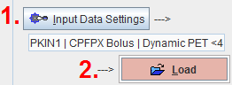
Input Data Settings
The first step consists of defining the image data set with the Input Data Setting button. It opens a window which allows switching between the different data formats and selecting one or multiple image series, depending on the model. The lower part of the window serves for the specification of data transformations during loading.
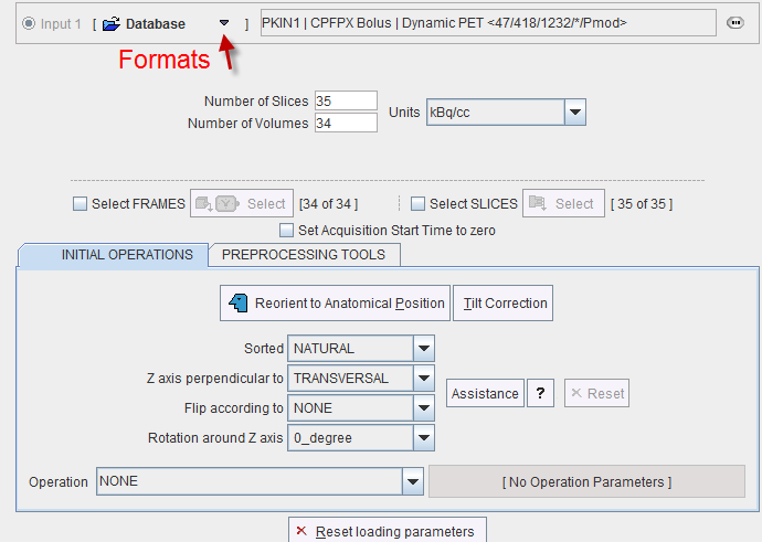
It is the standard image loading dialog which changes according to the format of the image data. When the FRAMES or the SLICES boxes are checked, image loading can be restricted to a sub-range using the corresponding Select buttons. In the lower part of the dialog window, image processing options can be specified which will be applied during loading.
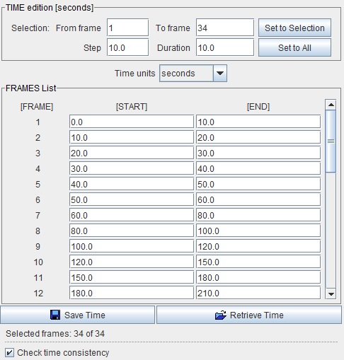
It is very important that the acquisition timing is correct when loading dynamic series. For formats which have this information defined in the file (such as DICOM) the Times box does not become active. Otherwise, the user needs to activate the Edit Time button. A dialog window is then shown in which the frame START and END times can be modified.
Notes:
1. The data loader always retains the definition of the last successful loading operation. This is important when working with data formats which do not include time and unit information, or if image processing options have been applied such as smoothing.
2. The fastest way to reset all operations is using the Reset loading parameters button.
3. Image data without timing information should be avoided in PXMOD. In such cases it is recommended to convert the data to a format with full timing support and proper frame times. Wrong timing will in many cases produce erroneous results.
Data Loading
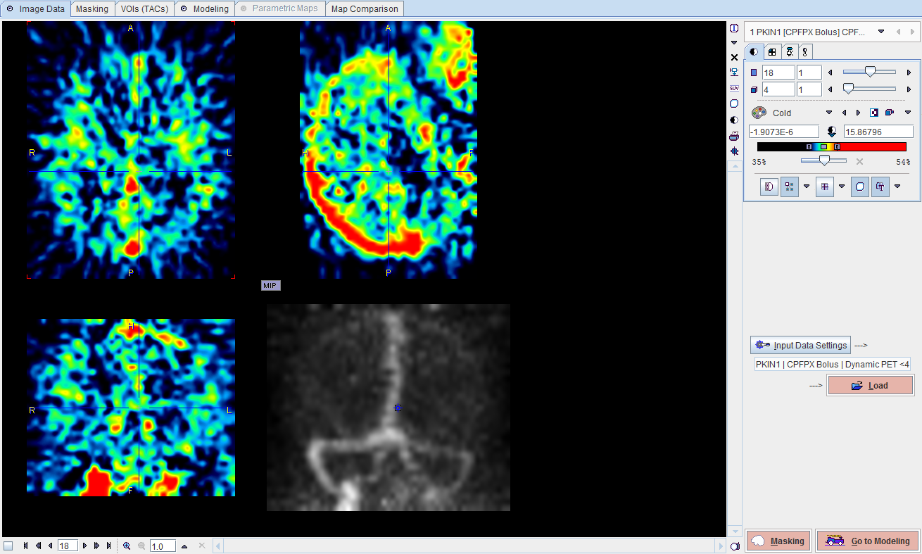
A description of the selected image is shown in the text field underneath the Input Data Setting button. The actual image loading is finally performed with the red Load button.
The advantage of this organization is that the data configuration can be maintained between sessions, when creating new workspaces, and when switching models.
How To Continue
There are two ways to continue. If you do not want to create a mask or outline VOIs then use the Modeling button to proceed to the Modeling page. Otherwise select the Masking button.
Initially the Masking page appears with the loaded images in the left display area.
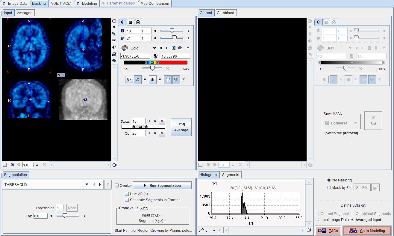
Averaging Frames
To obtain an appropriate data set for masking it is recommended to average the dynamic frames within an appropriate range. The range can be specified by the From and To numbers or using the slider handles. When the Average button is activated, the average uptake in the specified frame range is calculated and the result image shown on the Averaged sub-pane.
Segmentation for Creating a Mask
The next step consists of generating segments which represent tissues of interest. The segments can then be combined into a single mask. Segmentation can be performed on the Averaged images, but also on the dynamic Input series, depending on which tab is selected. The Histogram of the pixel values is updated according to the selected images.
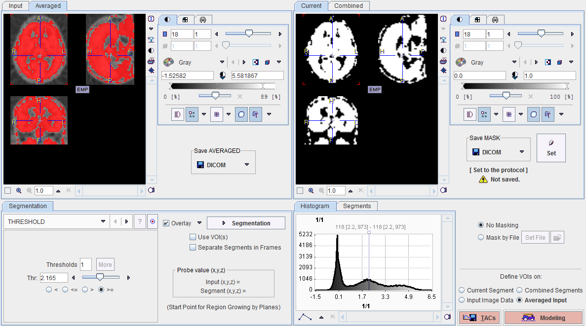
It is recommended to change the color table to Gray, and to enable the Overlay. Then, select one of the segmentation methods (described below) to specify an inclusion criterion. The pixels which satisfy the criterion are colored in red in the image overlay. Note that overlay updating might be slow when changing a segmentation parameter, depending on the segmentation method. Run Segmentation performs the actual segmentation and shows the result in the Current tab to the right. While standard segmentations create binary images with 0 (background) and 1 (segment) pixel values, there are clustering approaches which generate multiple segments in a single calculation. These segments are distinguished by increasing integer pixel values. Each Run Segmentation activation overrides the previous contents in Current.
Multiple segments can be combined into a mask. To prepare such a combination, copy promising segments to the Combined tab using the Set button to the right of SAVE MASK. As soon as the first segment has been copied, the button's name changes to Append. By repeated Run Segmentation and Append operations a list of segments can be built up in the Segments pane as illustrated below.
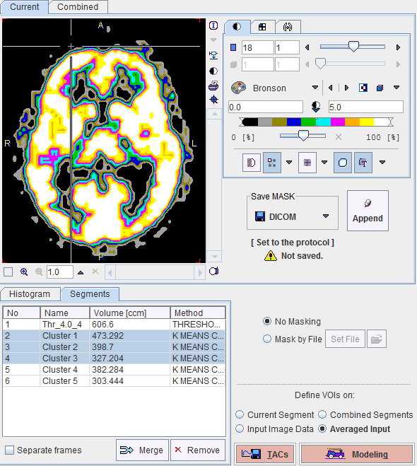
The No entry in the Segments list indicates the number by which a segment is identified in the Combined image, Name provides some descriptive information, Volume its physical volume, and Method identifies the applied segmentation method. Multiple segments in the list can be selected and transformed into a single segment by the Merge button. Hereby, the initially distinct values are replaced by a common value, and the original list entries deleted.
Saving the Mask for Model Processing
In order to use a generated segment image as a mask in model processing it must be saved as a file and configured. Saving can be performed using the Save MASK button in any of the supported image formats. Note that automatically the mask configuration button switches from No Masking to Mask by File, and the saved file is configured.
If a mask file already exists, the interactions described above are not necessary and it can be simply configured with the Set File button. The button next to Set File can be used to load the specified mask and show it in the Combined pane.
The Save MASK function can be applied on the Current or on the Combined panes. The corresponding image are saved as a mask.
Note that the saved mask is not binary in the case of multiple segments, so that the segments can be recovered. However, during the pixel-wise calculation only the non-zero mask pixels will be processed, while the other pixels are blanked.
How To Continue
There are two ways to continue. If you do not want to outline VOIs then use the Modeling button to proceed to the Modeling page. Otherwise first configure the image on which the VOIs should be outlined (Current Segment, Combined Segments, Input Image Data, Averaged Input), and then select the TACs button.