Residual Weighting

Residual Weighting in PKIN

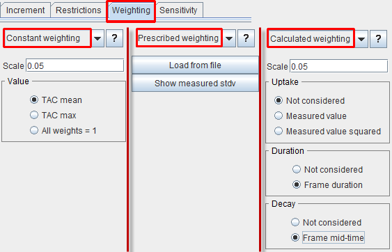
In PKIN, several different weight definitions are supported. They can be specified on the Weighting pane using the list selection with the three entries Constant weighting, Prescribed weighting and Calculated weighting. The contents of the different selections are illustrated in parallel below.

Weights Specifications

Constant
weighting

With constant weighting the same weight is applied to all residuals. Its size can be adjusted by the Scale factor and the radio button setting. In the case of TAC mean s_i is obtained as the average of all values in the TAC multiplied by the Scale factor. Similarly, with TAC max s_i is obtained as the maximal TAC value multiplied by the Scale value. With All weights = 1 the weights are all set equal to 1 independent of the Scale (s_i = s_i² = w_i = 1).

Prescribed
weighting

The default behavior of this method is to use the standard deviation of the pixel values in the VOI for calculating the TAC for weighting. This information is automatically available if the TACs have been sent from the PMOD viewing tool to PKIN, and can be visualized using the button Show measured stdv as illustrated below.

This definition can be overwritten by user-defined weights which are to be loaded with the Load stdv from file button. Please see below how the file has to be formatted.

Calculated
weighting

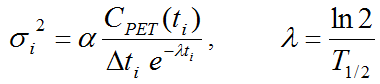
With this selection the variance is calculated for each TAC value from an equation which may take into account the measured uptake, the correction of the radioactive decay, and the duration of the acquisition. The full equation is as follows:

It includes a Scale factor a, the decay-corrected Uptake C_PET(t_i) at frame mid-time t_i, the frame Duration Dt_i, and the Decay constant l which is obtained from the half-life T_1/2 of the isotope.
The settings of the radio buttons have the following effect on the equation above for calculating s_i²:

Uptake:
Not considered: C_PET(t_i) is replaced by 1.
Measured value: C_PET(t_i) is used, corresponding to Poisson weighting. The effect is that more emphasis is given on low-uptake values than on high-uptake values. This may be helpful for example if the fit seems to not account enough for the tail of a decreasing function such as the input curve.
Measured value squared: C_PET(t_i) is replaced by C_PET²(t_i), corresponding to Relative weighting. With this option the influence of the uptake is further increased. It should be used with care because by squaring small uptake values (<<1) very small variances are generated which transform into heavy weighting. As a consequence, a few small uptake values may have too much impact on the fit.
Duration:
Not considered: Dt_i is replaced by 1.
Measured value: The individual frame durations Dt_i are used, so that longer acquisitions are considered more reliable.
Decay:
Not considered: is replaced by 1.
Frame mid-time: is used, so that earlier acquisitions are considered more reliable.

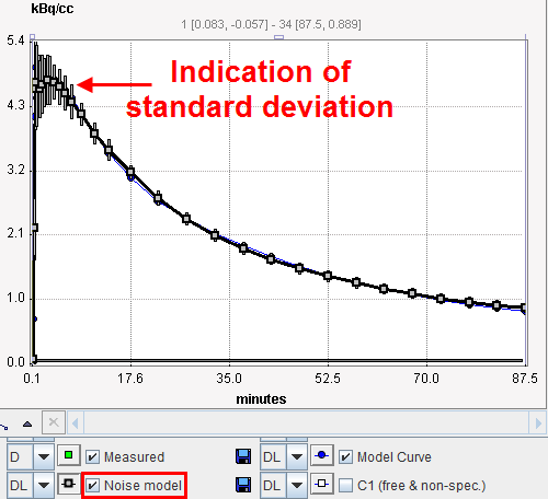
Each time the configuration is changed, the standard deviation s_i is calculated and plotted as an error bar around the measurements. This feedback gives the user a visual feedback as a help in judging the adequacy of the specified weighting.

Measured Standard Deviation

Loading Externally Defined Weights

Some users might want to implement their own residual weighting schemes. To this end they should calculate the standard deviations s_i for the different acquisition frames from which the weights will be calculated according to

The s_i should be prepared in a tab-delimited text file of the following form:

t[seconds]		standard-dev[kBq/cc]
10		0.10300076
30		0.01717448
50		0.01195735
70		0.01010257
etc		...

The header line is required. The first column represents the frame mid-times (although the values are not interpreted), and the second column the standard deviations in appropriate units. The number of entries must be equal the number of acquisitions, and the columns separated by spaces or tabs. For example, such a file can be prepared in MS Excel and then saved as a text file with tab delineation.

This definition can be loaded by the Load stdv from file button available with Prescribed weighting.

Display of the Residuals

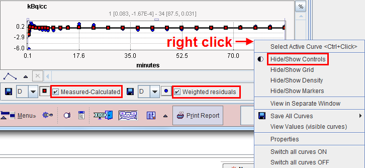
The curve area with the residuals contains the information of the raw unweighted as well as the weighted residuals. The context menu as illustrated below (right mouse click into the curve area) can be employed for showing/hiding the curve controls and using them for changing the displayed information.

Use of the Weights in Monte Carlo Simulations

Monte Carlo simulations require the generation of noise which is defined by a distribution type as well as its deviation characteristics. Assuming that the weights specification corresponds to the standard deviation of the measurement noise, the regional weighting specification is used in the Monte Carlo noise generation together with the distribution type. Note that the Scale factor has no impact on fitting, but that it is highly relevant in Monte Carlo simulations.