![]()
![]()
![]()
![]()
|
|
|
|
|
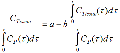
In 2010 Ito et al. introduced a new graphical method for the analysis of receptor ligand binding [62]. It is applied with a plasma input curve for the calculation of the total distribution volume Vt, the distribution volume of the nondisplaceable compartment VND, and therefore also allows calculation of the binding potential BPND. Furthermore, the shape of the plot gives an indication whether there is specific binding or not not.
The equation of the graphical plot called is given by the equation
The following cases can be distinguished:
Implementation Notes
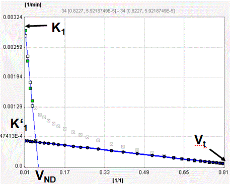
The Ito Plot model calculates and displays the measurements transformed as described by the Ito plot formula above. It allows fitting two regression lines as follows:
If any of the times is changed to define a new data segment, the program finds the closest acquisition start time, fits the two regression lines, and updates the calculated parameters.
Per default, only the Ito Plot and the late regression line is shown in the curve area. However, the early regression line can also be visualized as illustrated above by enabling its box in the curve control area.
Ito Plot Publication, Abstract [62]
"In positron emission tomography (PET) studies with radioligands for neuroreceptors, tracer kinetics have been described by the standard two-tissue compartment model that includes the compartments of nondisplaceable binding and specific binding to receptors. In the present study, we have developed a new graphic plot analysis to determine the total distribution volume (V(T)) and nondisplaceable distribution volume (V(ND)) independently, and therefore the binding potential (BP(ND)). In this plot, Y(t) is the ratio of brain tissue activity to time-integrated arterial input function, and X(t) is the ratio of time-integrated brain tissue activity to time-integrated arterial input function. The x-intercept of linear regression of the plots for early phase represents V(ND), and the x-intercept of linear regression of the plots for delayed phase after the equilibrium time represents V(T). BP(ND) can be calculated by BP(ND)=V(T)/V(ND)-1. Dynamic PET scanning with measurement of arterial input function was performed on six healthy men after intravenous rapid bolus injection of [(11)C]FLB457. The plot yielded a curve in regions with specific binding while it yielded a straight line through all plot data in regions with no specific binding. V(ND), V(T), and BP(ND) values calculated by the present method were in good agreement with those by conventional non-linear least-squares fitting procedure. This method can be used to distinguish graphically whether the radioligand binding includes specific binding or not."