Processing Overview
Data processing of studies with PET or SPECT tracers typically consists of the following parts:
1. Data Loading
|
- Create a new data set.
- Load the whole blood curve (total activity concentration of tracer in the blood samples).
- Load the plasma activity curve. Depending on the preparation of the blood data the plasma activity curve can represent
the unchanged tracer (parent) in plasma, or total tracer in the plasma of the blood samples including the metabolites. In the case of total tracer the metabolite correction has to be performed in PKIN. - An alternative to loading the plasma activity curve is loading the plasma fraction curve. In this case the total plasma activity is calculated by multiplying whole blood activity with the plasma fraction.
- Load the parent fraction curve (fraction of unchanged tracer in plasma). This is only necessary if the loaded plasma curve represents total tracer activity in plasma including metabolites.
- Load the average time-activity curves of one or multiple tissue regions.
|
2. Input Curve Configuration
|
- Define interpolation functions (called models) for the different types of blood data and fit them to the data.
- The input curve is obtained as the multiplication of the plasma model with the parent fraction model.
|
3. Kinetic Model Configuration
|
- Select a region with a "typical" time-activity curve (TAC) from the Region list.
- Select a simple model from the Model list.
- Enable the parameters to be fitted by checking their boxes; unchecked parameters remain at the initial values entered.
- Select a weighting scheme of the residuals; variable or constant (default) weighting is available.
|
4. Kinetic Model Fitting
|
- Fit the model parameters by activating the Fit current region button.
- Consult the residuals to check whether the model is adequate; there should ideally be no bias in the residuals, just random noise.
- If the model is fine, configure Copy the model to all regions to Model & Par, activate the button to establish then save initial model configuration for all TACs, then activate Fit all regions.
- Check the fit result for all the TACs.
- If the model is not yet fine, test more complex models.
|
5. Kinetic Model Comparison
|
- Switch between compartment models of different complexity and fit. The parameters are either maintained for each model type, or converted, according to the Model conversion setting in the Menu.
- Check the residuals for judging model adequacy.
- Check the different criteria on the Details tab (Schwartz Criterion SC, Akaike Information Criterion AIC, Model Selection Criterion MSC) to decide whether a more complex model is supported by the data.
- Check for parameter identifiability. As an indicator of the parameter standard errors (%SE) are returned from the fit. They should remain limited for all relevant parameters. Additionally, Monte Carlo simulations can be performed to obtain statistics of the parameter estimates.
- If justified by physiology, try to improve the stability of parameter estimation by enforcing common parameters among regions in a coupled fitting procedure.
- Compare the outcome of compartment models with that of other models, such as reference models or graphical plots.
|
6. Saving
|
- Save all model information together with the data in a composite text .km file which allows restoring a session.
- Save a summary of all regional parameters in an EXCEL-ready text file .kinPar.
|
7. Batch Processing
|
Lengthy calculations such as coupled fits with many regional TACs or Monte Carlo simulations can be run in a batch job. The results are saved both as .km files and in an EXCEL-ready text file.
|
Starting the Kinetic Modeling Tool
The kinetic modeling tool is started with the Kinetic button from the PMOD ToolBox

or by directly dragging kinetic modeling (.km) files onto the above button.
The user interface is organized as illustrated below. The left part of the display visualizes the data, the model and the fit. The green squares represent the tissue measurement values (tissue time-activity curve, TAC), the red circles the input curve, the yellow circles the blood spillover curve (whole blood time-activity curve), and the blue circles the calculated model curve with the current model configuration shown to the right. The lower curve display shows the residuals, i.e. the difference between the measurement and the model curve. Weighted and unweighted residuals can be shown.
The right part gives access to the different operations which are described in the following sections.
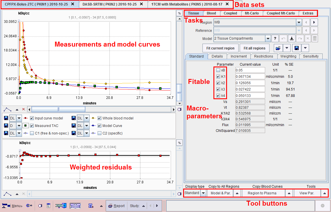
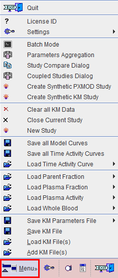
The Menu is located in the lower left corner and is used for data operations such as loading, saving or closing.
Loaded data sets can be added into new tabs, so multiple data sets can be available simultaneously and selected for processing using the named tabs.